05 - Arima

Introducing Arima - Autoregressive Integrated Moving Average.
Time-Series
ARIMA
Decomposition
Author

François de Ryckel

Published

January 9, 2024

Modified

January 22, 2024

Introduction

This post is about introducing ARIMA using the CPI data and various R framework for time series. Autoregressive because it is based on past value and moving average to smooth the time series data.

Our previous post on autocorrelation and partial autocorelation could be considered as prior material.

Autoregression is a class of linear model where the outcome variable is regressed on its previous values (lagged observations). \[Y_t = \delta + \phi_1 Y_{t-1} + \phi_2 Y_{t-2} + \cdots + \phi_p Y_{t-p} + \epsilon_t\] This AR model used \(p\) lags, hence we say it is of order \(p\).

  • \(\delta\) is an intercept like term
  • \(Y_{t-i}\) are the regressors (time series own lagged observations) with parameters \(\phi_{t-i}\)
  • \(\epsilon\) is the error term

Moving Average (MA) is another class of linear model where the outcome variable is regressed using its own previous error terms. \[Y_t = \mu + \theta_1 \epsilon_{t-1} + \theta_2 \epsilon_{t-2} + \cdots + \theta_q \epsilon_{t-q} + \epsilon_t\] This MA model used \(q\) lags, hence we say it is of order \(q\).

Putting it all together, the outcome variable of an ARIMA model can be predicted: \[Y_t = \{\delta + \phi_1 Y_{t-1} + \phi_2 Y_{t-2} + \cdots + \phi_p Y_{t-p} + \epsilon_t \} + \{\mu + \theta_1 \epsilon_{t-1} + \theta_2 \epsilon_{t-2} + \cdots + \theta_q \epsilon_{t-q} + \epsilon_t \}\] This can be simplify into: \[Y_t = \delta + \sum_{i=1}^p \phi_i Y_{t-i} + \sum_{j=1}^q \theta_j \epsilon_{t-j} + \epsilon_t\]

The parameters of an ARIMA model are (p, d, q) :

  • \(p\) - Autoregressive. The number of lagged observations in the model. Use the previous \(n\) observations as predictors.
  • \(d\) - Integrated. The number of times the data is differenced to make the data stationary
  • \(q\) - the size of the moving average. Use previous errors to predict \(Y_t\)

To apply an ARIMA model to a set of data, we will use the US CPI Energy component that we downloaded on the FED St-Louis website.

Application using R

library(readr)
library(dplyr)
library(ggplot2)
library(modeltime)
library(timetk)

df <- read_csv('../../../raw_data/CPI_energy.csv') |> 
  select(date = DATE, cpi_energy = CPIENGNS)
glimpse(df)
Rows: 803
Columns: 2
$ date       <date> 1957-01-01, 1957-02-01, 1957-03-01, 1957-04-01, 1957-05-01…
$ cpi_energy <dbl> 21.3, 21.5, 21.6, 21.5, 21.4, 21.4, 21.5, 21.4, 21.5, 21.4,…

ARIMA using the base R framework

We need first to convert our df into a ts object.

df_ts <- ts(df$cpi_energy, start = c(1957,01), frequency = 12, end = c(2023, 11))
str(df_ts)
 Time-Series [1:803] from 1957 to 2024: 21.3 21.5 21.6 21.5 21.4 21.4 21.5 21.4 21.5 21.4 ...
ts.plot(df_ts, xlab = 'Date', ylab = 'Energy CPI')

It is usually a wise idea to check for outliers? An easy way to do this is using a boxplot.

boxplot(df_ts)

We use the ACF to determine the MA parameter (q) of the ARIMA model.

  • Significant spikes at specific lags in the ACF plot suggest potential MA terms at those lags
  • An ACF plot that cuts off sharply after a few lags often indicates a suitable MA model
acf(df_ts, lag.max = 100)

ggacf(df_ts, num_lags = 100)

Data is clearly not stationary. We will need to use differentiation to make it stationary.

The PCAF helps determine the AR (Autoregressive) order (p) in an ARIMA model.

  • Significant spikes at specific lags in the PACF plot suggest potential AR terms at those lags
  • A PACF plot that cuts off sharply after a few lags often indicates a suitable AR model
pacf(df_ts, lag.max = 100)

This can be confirm with Augmented Dickey Fuller test

tseries::adf.test(df_ts)
Registered S3 method overwritten by 'quantmod':
  method            from
  as.zoo.data.frame zoo 

    Augmented Dickey-Fuller Test

data:  df_ts
Dickey-Fuller = -2.4123, Lag order = 9, p-value = 0.4038
alternative hypothesis: stationary

adf test confirm non-stationarity of our ts. We can differentiate our ts to make it stationary.

diff_ts <- diff(x = df_ts, lag = 1)
ts.plot(diff_ts)

tseries::adf.test(diff_ts)
Warning in tseries::adf.test(diff_ts): p-value smaller than printed p-value

    Augmented Dickey-Fuller Test

data:  diff_ts
Dickey-Fuller = -9.4624, Lag order = 9, p-value = 0.01
alternative hypothesis: stationary

We can create our training and testing set.

train_ts <- df_ts[1:793]

We can now use ARIMA model using 1 and 1 for parameter (all we could see from acf)

result <- arima(train_ts, order = c(0, 1, 2))
result

Call:
arima(x = train_ts, order = c(0, 1, 2))

Coefficients:
         ma1     ma2
      0.5197  0.0884
s.e.  0.0356  0.0361

sigma^2 estimated as 17.24:  log likelihood = -2251.54,  aic = 4509.07
tsdiag(result)

predict(result, 3)
$pred
Time Series:
Start = 794 
End = 796 
Frequency = 1 
[1] 290.5702 292.0037 292.0037

$se
Time Series:
Start = 794 
End = 796 
Frequency = 1 
[1]  4.152615  7.554318 10.082648
result_df <- arima(df_ts, order = c(0, 1, 2))
result_df

Call:
arima(x = df_ts, order = c(0, 1, 2))

Coefficients:
         ma1     ma2
      0.5033  0.0834
s.e.  0.0347  0.0358

sigma^2 estimated as 17.52:  log likelihood = -2286.24,  aic = 4578.49
predict(result_df, 2)
$pred
          Jan Feb Mar Apr May Jun Jul Aug Sep Oct Nov      Dec
2023                                                  273.7094
2024 273.2768                                                 

$se
          Jan Feb Mar Apr May Jun Jul Aug Sep Oct Nov      Dec
2023                                                  4.185297
2024 7.556805                                                 
result_df <- arima(df_ts, order = c(4, 1, 1))
result_df

Call:
arima(x = df_ts, order = c(4, 1, 1))

Coefficients:
         ar1      ar2     ar3      ar4      ma1
      1.1419  -0.4870  0.1896  -0.1582  -0.6576
s.e.  0.0776   0.0626  0.0531   0.0362   0.0722

sigma^2 estimated as 16.92:  log likelihood = -2272.35,  aic = 4556.69
predict(result_df, 2)
$pred
          Jan Feb Mar Apr May Jun Jul Aug Sep Oct Nov      Dec
2023                                                  272.8635
2024 270.8238                                                 

$se
          Jan Feb Mar Apr May Jun Jul Aug Sep Oct Nov      Dec
2023                                                  4.112985
2024 7.361178                                                 
forecast::auto.arima(df_ts, trace = T, stepwise = F, approximation = F)

 ARIMA(0,1,0)                               : 4762.801
 ARIMA(0,1,0)            with drift         : 4761.123
 ARIMA(0,1,0)(0,0,1)[12]                    : 4751.105
 ARIMA(0,1,0)(0,0,1)[12] with drift         : 4750.212
 ARIMA(0,1,0)(0,0,2)[12]                    : 4749.802
 ARIMA(0,1,0)(0,0,2)[12] with drift         : 4749.14
 ARIMA(0,1,0)(1,0,0)[12]                    : 4748.883
 ARIMA(0,1,0)(1,0,0)[12] with drift         : 4748.184
 ARIMA(0,1,0)(1,0,1)[12]                    : Inf
 ARIMA(0,1,0)(1,0,1)[12] with drift         : Inf
 ARIMA(0,1,0)(1,0,2)[12]                    : Inf
 ARIMA(0,1,0)(1,0,2)[12] with drift         : Inf
 ARIMA(0,1,0)(2,0,0)[12]                    : 4742.386
 ARIMA(0,1,0)(2,0,0)[12] with drift         : 4742.203
 ARIMA(0,1,0)(2,0,1)[12]                    : Inf
 ARIMA(0,1,0)(2,0,1)[12] with drift         : Inf
 ARIMA(0,1,0)(2,0,2)[12]                    : Inf
 ARIMA(0,1,0)(2,0,2)[12] with drift         : Inf
 ARIMA(0,1,1)                               : 4581.902
 ARIMA(0,1,1)            with drift         : 4581.821
 ARIMA(0,1,1)(0,0,1)[12]                    : 4577.654
 ARIMA(0,1,1)(0,0,1)[12] with drift         : 4577.884
 ARIMA(0,1,1)(0,0,2)[12]                    : 4573.756
 ARIMA(0,1,1)(0,0,2)[12] with drift         : 4574.212
 ARIMA(0,1,1)(1,0,0)[12]                    : 4576.446
 ARIMA(0,1,1)(1,0,0)[12] with drift         : 4576.758
 ARIMA(0,1,1)(1,0,1)[12]                    : Inf
 ARIMA(0,1,1)(1,0,1)[12] with drift         : Inf
 ARIMA(0,1,1)(1,0,2)[12]                    : Inf
 ARIMA(0,1,1)(1,0,2)[12] with drift         : Inf
 ARIMA(0,1,1)(2,0,0)[12]                    : 4568.379
 ARIMA(0,1,1)(2,0,0)[12] with drift         : 4569.08
 ARIMA(0,1,1)(2,0,1)[12]                    : Inf
 ARIMA(0,1,1)(2,0,1)[12] with drift         : Inf
 ARIMA(0,1,1)(2,0,2)[12]                    : Inf
 ARIMA(0,1,1)(2,0,2)[12] with drift         : Inf
 ARIMA(0,1,2)                               : 4578.515
 ARIMA(0,1,2)            with drift         : 4578.734
 ARIMA(0,1,2)(0,0,1)[12]                    : 4575.644
 ARIMA(0,1,2)(0,0,1)[12] with drift         : 4576.08
 ARIMA(0,1,2)(0,0,2)[12]                    : 4572.671
 ARIMA(0,1,2)(0,0,2)[12] with drift         : 4573.279
 ARIMA(0,1,2)(1,0,0)[12]                    : 4574.772
 ARIMA(0,1,2)(1,0,0)[12] with drift         : 4575.261
 ARIMA(0,1,2)(1,0,1)[12]                    : Inf
 ARIMA(0,1,2)(1,0,1)[12] with drift         : Inf
 ARIMA(0,1,2)(1,0,2)[12]                    : Inf
 ARIMA(0,1,2)(1,0,2)[12] with drift         : Inf
 ARIMA(0,1,2)(2,0,0)[12]                    : 4568.289
 ARIMA(0,1,2)(2,0,0)[12] with drift         : 4569.079
 ARIMA(0,1,2)(2,0,1)[12]                    : Inf
 ARIMA(0,1,2)(2,0,1)[12] with drift         : Inf
 ARIMA(0,1,3)                               : 4579.677
 ARIMA(0,1,3)            with drift         : 4580.023
 ARIMA(0,1,3)(0,0,1)[12]                    : 4577.191
 ARIMA(0,1,3)(0,0,1)[12] with drift         : 4577.708
 ARIMA(0,1,3)(0,0,2)[12]                    : 4574.269
 ARIMA(0,1,3)(0,0,2)[12] with drift         : 4574.946
 ARIMA(0,1,3)(1,0,0)[12]                    : 4576.379
 ARIMA(0,1,3)(1,0,0)[12] with drift         : 4576.941
 ARIMA(0,1,3)(1,0,1)[12]                    : Inf
 ARIMA(0,1,3)(1,0,1)[12] with drift         : Inf
 ARIMA(0,1,3)(2,0,0)[12]                    : 4569.998
 ARIMA(0,1,3)(2,0,0)[12] with drift         : 4570.839
 ARIMA(0,1,4)                               : 4581.69
 ARIMA(0,1,4)            with drift         : 4582.053
 ARIMA(0,1,4)(0,0,1)[12]                    : 4579.221
 ARIMA(0,1,4)(0,0,1)[12] with drift         : 4579.733
 ARIMA(0,1,4)(1,0,0)[12]                    : 4578.408
 ARIMA(0,1,4)(1,0,0)[12] with drift         : 4578.96
 ARIMA(0,1,5)                               : 4583.72
 ARIMA(0,1,5)            with drift         : 4584.063
 ARIMA(1,1,0)                               : 4592.114
 ARIMA(1,1,0)            with drift         : 4592.78
 ARIMA(1,1,0)(0,0,1)[12]                    : 4590.795
 ARIMA(1,1,0)(0,0,1)[12] with drift         : 4591.591
 ARIMA(1,1,0)(0,0,2)[12]                    : 4589.897
 ARIMA(1,1,0)(0,0,2)[12] with drift         : 4590.8
 ARIMA(1,1,0)(1,0,0)[12]                    : 4590.336
 ARIMA(1,1,0)(1,0,0)[12] with drift         : 4591.158
 ARIMA(1,1,0)(1,0,1)[12]                    : Inf
 ARIMA(1,1,0)(1,0,1)[12] with drift         : Inf
 ARIMA(1,1,0)(1,0,2)[12]                    : Inf
 ARIMA(1,1,0)(1,0,2)[12] with drift         : Inf
 ARIMA(1,1,0)(2,0,0)[12]                    : 4587.308
 ARIMA(1,1,0)(2,0,0)[12] with drift         : 4588.314
 ARIMA(1,1,0)(2,0,1)[12]                    : Inf
 ARIMA(1,1,0)(2,0,1)[12] with drift         : Inf
 ARIMA(1,1,0)(2,0,2)[12]                    : Inf
 ARIMA(1,1,0)(2,0,2)[12] with drift         : Inf
 ARIMA(1,1,1)                               : 4577.984
 ARIMA(1,1,1)            with drift         : 4578.289
 ARIMA(1,1,1)(0,0,1)[12]                    : 4575.351
 ARIMA(1,1,1)(0,0,1)[12] with drift         : 4575.838
 ARIMA(1,1,1)(0,0,2)[12]                    : 4572.434
 ARIMA(1,1,1)(0,0,2)[12] with drift         : 4573.078
 ARIMA(1,1,1)(1,0,0)[12]                    : 4574.518
 ARIMA(1,1,1)(1,0,0)[12] with drift         : 4575.051
 ARIMA(1,1,1)(1,0,1)[12]                    : Inf
 ARIMA(1,1,1)(1,0,1)[12] with drift         : Inf
 ARIMA(1,1,1)(1,0,2)[12]                    : Inf
 ARIMA(1,1,1)(1,0,2)[12] with drift         : Inf
 ARIMA(1,1,1)(2,0,0)[12]                    : 4568.139
 ARIMA(1,1,1)(2,0,0)[12] with drift         : 4568.95
 ARIMA(1,1,1)(2,0,1)[12]                    : Inf
 ARIMA(1,1,1)(2,0,1)[12] with drift         : Inf
 ARIMA(1,1,2)                               : 4579.966
 ARIMA(1,1,2)            with drift         : 4580.292
 ARIMA(1,1,2)(0,0,1)[12]                    : 4577.355
 ARIMA(1,1,2)(0,0,1)[12] with drift         : 4577.857
 ARIMA(1,1,2)(0,0,2)[12]                    : 4574.418
 ARIMA(1,1,2)(0,0,2)[12] with drift         : 4575.085
 ARIMA(1,1,2)(1,0,0)[12]                    : 4576.524
 ARIMA(1,1,2)(1,0,0)[12] with drift         : 4577.071
 ARIMA(1,1,2)(1,0,1)[12]                    : Inf
 ARIMA(1,1,2)(1,0,1)[12] with drift         : Inf
 ARIMA(1,1,2)(2,0,0)[12]                    : 4570.12
 ARIMA(1,1,2)(2,0,0)[12] with drift         : 4570.951
 ARIMA(1,1,3)                               : 4581.695
 ARIMA(1,1,3)            with drift         : 4582.053
 ARIMA(1,1,3)(0,0,1)[12]                    : 4579.222
 ARIMA(1,1,3)(0,0,1)[12] with drift         : 4579.743
 ARIMA(1,1,3)(1,0,0)[12]                    : 4578.411
 ARIMA(1,1,3)(1,0,0)[12] with drift         : 4578.979
 ARIMA(1,1,4)                               : 4573.756
 ARIMA(1,1,4)            with drift         : 4571.09
 ARIMA(2,1,0)                               : 4579.505
 ARIMA(2,1,0)            with drift         : 4579.69
 ARIMA(2,1,0)(0,0,1)[12]                    : 4577.142
 ARIMA(2,1,0)(0,0,1)[12] with drift         : 4577.505
 ARIMA(2,1,0)(0,0,2)[12]                    : 4575.062
 ARIMA(2,1,0)(0,0,2)[12] with drift         : 4575.574
 ARIMA(2,1,0)(1,0,0)[12]                    : 4576.421
 ARIMA(2,1,0)(1,0,0)[12] with drift         : 4576.826
 ARIMA(2,1,0)(1,0,1)[12]                    : Inf
 ARIMA(2,1,0)(1,0,1)[12] with drift         : Inf
 ARIMA(2,1,0)(1,0,2)[12]                    : Inf
 ARIMA(2,1,0)(1,0,2)[12] with drift         : Inf
 ARIMA(2,1,0)(2,0,0)[12]                    : 4571.428
 ARIMA(2,1,0)(2,0,0)[12] with drift         : 4572.095
 ARIMA(2,1,0)(2,0,1)[12]                    : Inf
 ARIMA(2,1,0)(2,0,1)[12] with drift         : Inf
 ARIMA(2,1,1)                               : 4579.893
 ARIMA(2,1,1)            with drift         : 4580.248
 ARIMA(2,1,1)(0,0,1)[12]                    : 4577.321
 ARIMA(2,1,1)(0,0,1)[12] with drift         : 4577.839
 ARIMA(2,1,1)(0,0,2)[12]                    : 4574.356
 ARIMA(2,1,1)(0,0,2)[12] with drift         : 4575.04
 ARIMA(2,1,1)(1,0,0)[12]                    : 4576.493
 ARIMA(2,1,1)(1,0,0)[12] with drift         : 4577.055
 ARIMA(2,1,1)(1,0,1)[12]                    : Inf
 ARIMA(2,1,1)(1,0,1)[12] with drift         : Inf
 ARIMA(2,1,1)(2,0,0)[12]                    : 4570.052
 ARIMA(2,1,1)(2,0,0)[12] with drift         : 4570.9
 ARIMA(2,1,2)                               : 4581.576
 ARIMA(2,1,2)            with drift         : 4582.003
 ARIMA(2,1,2)(0,0,1)[12]                    : Inf
 ARIMA(2,1,2)(0,0,1)[12] with drift         : Inf
 ARIMA(2,1,2)(1,0,0)[12]                    : Inf
 ARIMA(2,1,2)(1,0,0)[12] with drift         : Inf
 ARIMA(2,1,3)                    : Inf
 ARIMA(2,1,3) with drift         : Inf
 ARIMA(3,1,0)                               : 4581.026
 ARIMA(3,1,0)            with drift         : 4581.307
 ARIMA(3,1,0)(0,0,1)[12]                    : 4578.438
 ARIMA(3,1,0)(0,0,1)[12] with drift         : 4578.91
 ARIMA(3,1,0)(0,0,2)[12]                    : 4575.713
 ARIMA(3,1,0)(0,0,2)[12] with drift         : 4576.374
 ARIMA(3,1,0)(1,0,0)[12]                    : 4577.627
 ARIMA(3,1,0)(1,0,0)[12] with drift         : 4578.148
 ARIMA(3,1,0)(1,0,1)[12]                    : Inf
 ARIMA(3,1,0)(1,0,1)[12] with drift         : Inf
 ARIMA(3,1,0)(2,0,0)[12]                    : 4571.48
 ARIMA(3,1,0)(2,0,0)[12] with drift         : 4572.324
 ARIMA(3,1,1)                               : 4581.285
 ARIMA(3,1,1)            with drift         : 4581.576
 ARIMA(3,1,1)(0,0,1)[12]                    : 4578.762
 ARIMA(3,1,1)(0,0,1)[12] with drift         : 4579.224
 ARIMA(3,1,1)(1,0,0)[12]                    : 4577.945
 ARIMA(3,1,1)(1,0,0)[12] with drift         : 4578.452
 ARIMA(3,1,2)                               : 4568.698
 ARIMA(3,1,2) with drift         : Inf
 ARIMA(4,1,0)                               : 4575.634
 ARIMA(4,1,0)            with drift         : 4575.534
 ARIMA(4,1,0)(0,0,1)[12]                    : 4574.175
 ARIMA(4,1,0)(0,0,1)[12] with drift         : 4574.312
 ARIMA(4,1,0)(1,0,0)[12]                    : 4573.622
 ARIMA(4,1,0)(1,0,0)[12] with drift         : 4573.812
 ARIMA(4,1,1)                               : 4556.801
 ARIMA(4,1,1)            with drift         : 4554.628
 ARIMA(5,1,0)                               : 4561.352
 ARIMA(5,1,0)            with drift         : 4560.508


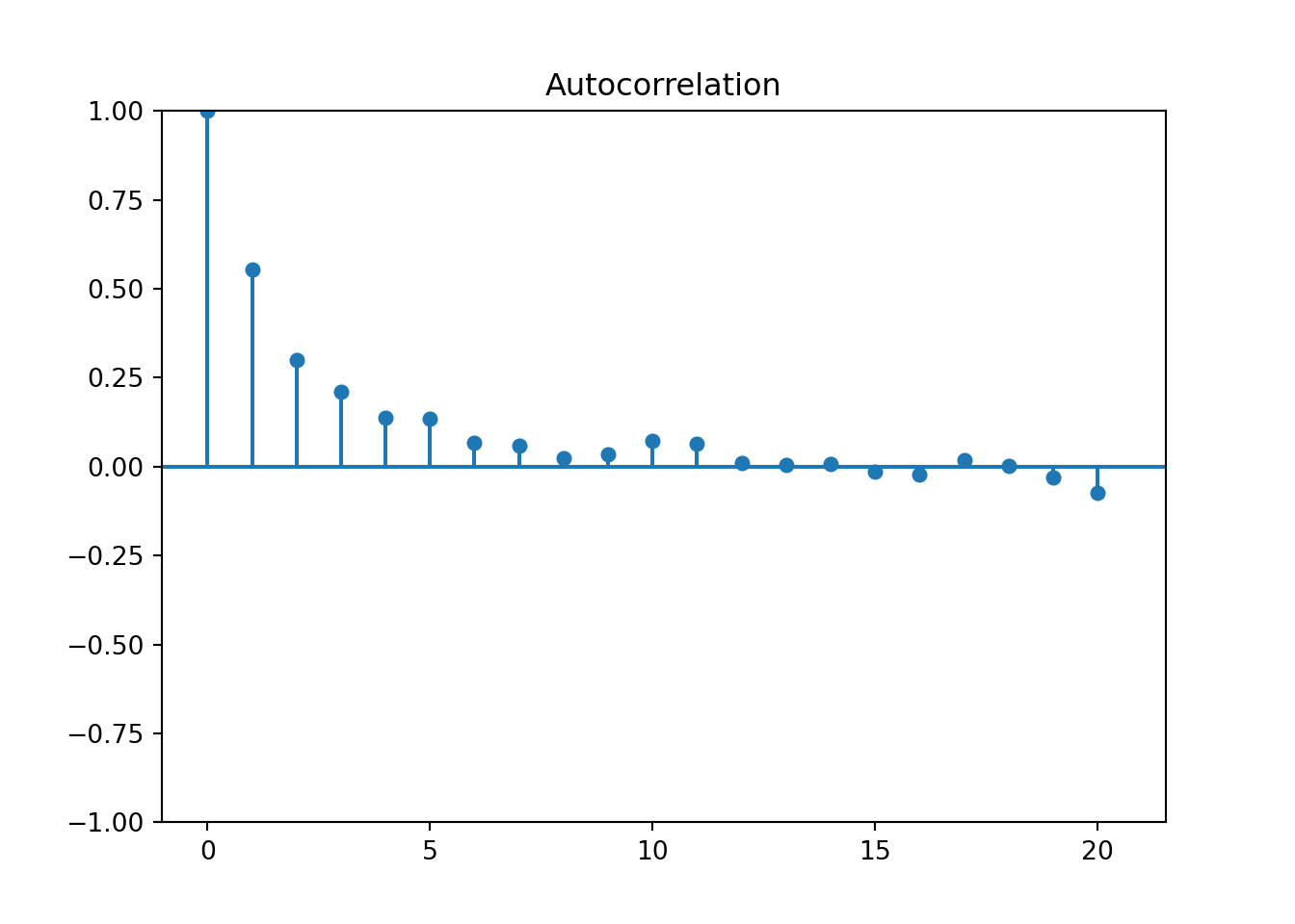
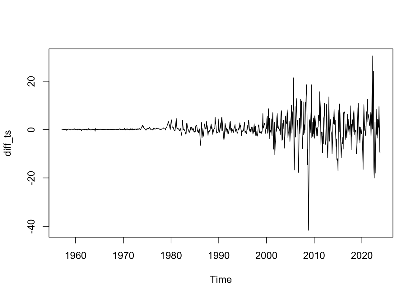
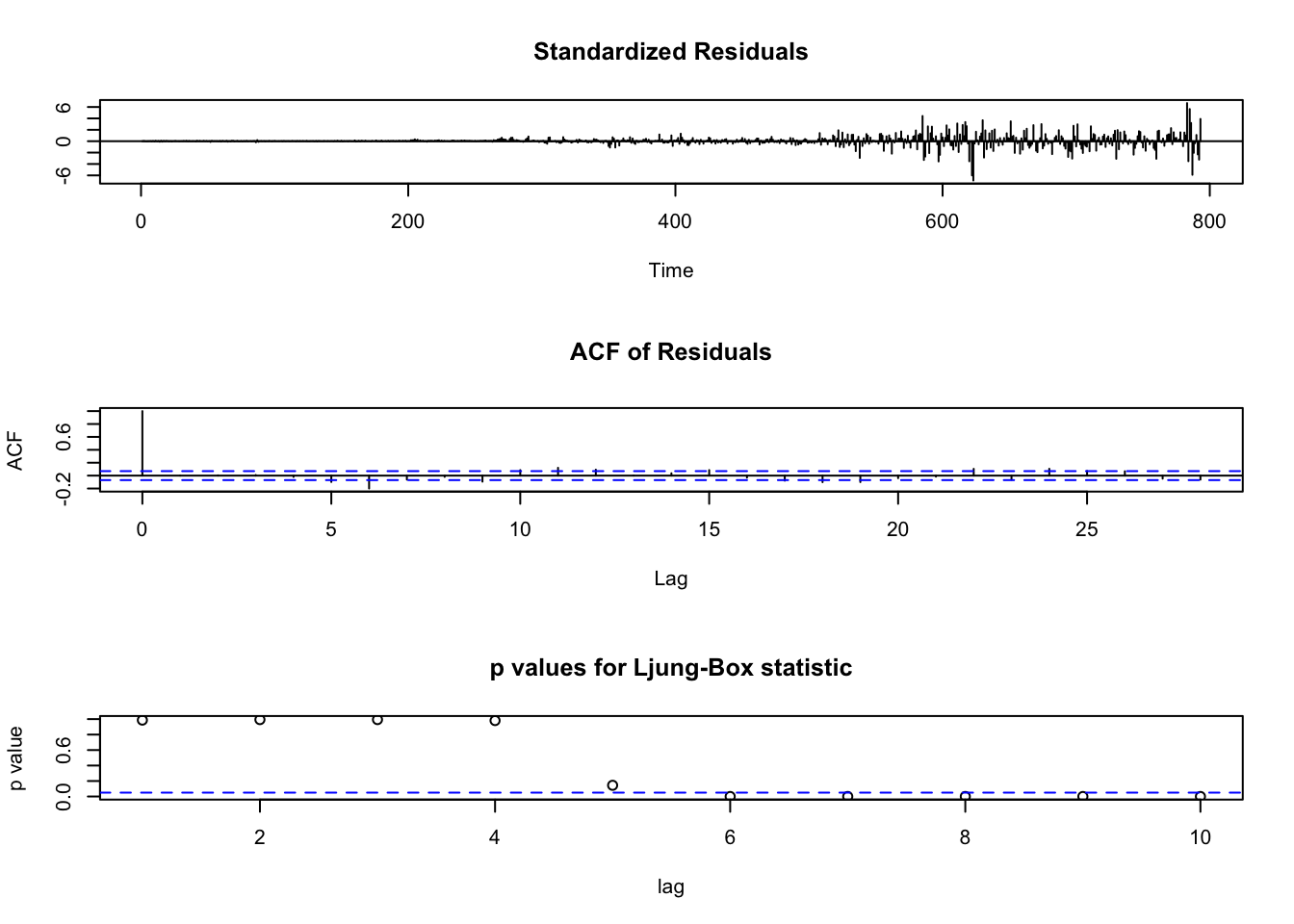
 Best model: ARIMA(4,1,1)            with drift         
Series: df_ts 
ARIMA(4,1,1) with drift 

Coefficients:
         ar1      ar2     ar3      ar4      ma1   drift
      1.1535  -0.4942  0.1912  -0.1603  -0.6749  0.3205
s.e.  0.0758   0.0622  0.0534   0.0365   0.0703  0.1523

sigma^2 = 16.95:  log likelihood = -2270.24
AIC=4554.49   AICc=4554.63   BIC=4587.3

Using modeltime framework

df |> plot_time_series(date, cpi_energy, .interactive = FALSE)

with model time, it is pretty easy to do get the value for arima.

cv_splits <- df |> 
  time_series_split(date_var = date, assess = '13 months', cumulative = TRUE)

cv_splits |> 
  tk_time_series_cv_plan() |>
  plot_time_series_cv_plan(.date_var = date, .value = cpi_energy, .interactive = FALSE)

library(tidymodels)
── Attaching packages ────────────────────────────────────── tidymodels 1.2.0 ──
✔ broom        1.0.5      ✔ rsample      1.2.1 
✔ dials        1.2.1      ✔ tibble       3.2.1 
✔ infer        1.0.7      ✔ tidyr        1.3.1 
✔ modeldata    1.3.0      ✔ tune         1.2.1 
✔ parsnip      1.2.1      ✔ workflows    1.1.4 
✔ purrr        1.0.2      ✔ workflowsets 1.1.0 
✔ recipes      1.0.10     ✔ yardstick    1.3.1 
── Conflicts ───────────────────────────────────────── tidymodels_conflicts() ──
✖ purrr::discard()  masks scales::discard()
✖ dplyr::filter()   masks stats::filter()
✖ dplyr::lag()      masks stats::lag()
✖ yardstick::spec() masks readr::spec()
✖ recipes::step()   masks stats::step()
• Learn how to get started at https://www.tidymodels.org/start/
library(parsnip)
library(modeltime)

model_fit_arima <- arima_reg() |> 
  set_engine('auto_arima') |>
  fit(cpi_energy ~ date, training(cv_splits))
frequency = 12 observations per 1 year
model_fit_arima
parsnip model object

Series: outcome 
ARIMA(0,1,2)(0,0,2)[12] 

Coefficients:
         ma1     ma2    sma1    sma2
      0.5229  0.0895  0.0733  0.0907
s.e.  0.0356  0.0358  0.0400  0.0359

sigma^2 = 16.45:  log likelihood = -2222.54
AIC=4455.07   AICc=4455.15   BIC=4478.42