05 - Trinomials models for Quantitative Finance

Transition Density Function

library(tibble)     # tibble()
library(dplyr)      # mutate()
library(ggplot2)    # ggplot()

Setting the stage

A discrete random variable (DRV) $y$ can either go up with a probability of $\alpha$ or down with a probability of $\alpha$ or stay the same with a probability of $1-2\alpha$.

We call that a trinomial walk.

Generating an instance of a trinomial walk

alpha <- 0.3     # probability to go up or down 
                 # Hence, prob to stay the same is 0.4

#let's do a 252 steps trinomial walk (aka a year of daily movement). 

num_steps <- 252
prob <- runif(num_steps)

df <- tibble(step = 1:num_steps, prob = prob) |> 
  mutate(direction = if_else(prob < alpha, -1, if_else(prob > (1 - alpha), 1, 0)), 
         cum_walk = cumsum(direction))

ggplot(df, aes(x = step, y = cum_walk)) + 
  geom_line() + 
  ggtitle(label = 'Instance of a trinomial walk', subtitle = 'with 252 steps and symetric move') + 
  ylab(label = 'Cumulative distance')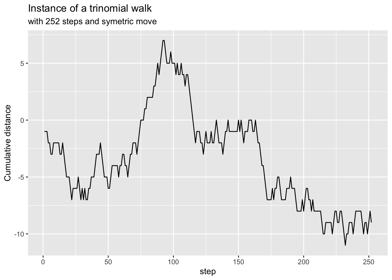

This is just one instance of a trinomial walk. In reality, we are interested in getting to know the probabilistic properties of the $y$ variable.

Deriving the Forward equation

$$\begin{array}{}\text{(1)}& Prob(a<y^{\prime }<b\text{ at time t’ }|\text{ y at time t})={\int }_a^{b}p(y,t;y^{\prime },t^{\prime })d{y}^{\prime }\end{array}$$

This (Equation 1) means: What is the probability that the random variable y’ lies between a and b at time t’ given it was at y at time t? In this case (y, t) are given, they are constant, they are known; while (y’, t’) are the variables.

We re-write this (Equation 1) for conciseness as $P(y,t;y^{\prime },t^{\prime })$.

Hence, another way to write (Equation 1) is $$\begin{array}{}\text{(2)}& P(y,t;y^{\prime },t^{\prime })=\alpha \cdot P(y,t;y^{\prime }+\delta y,t^{\prime }-\delta t)+(1-2\alpha )P(y,t;y^{\prime },t^{\prime }-\delta t)+\alpha \cdot P(y,t;y^{\prime }-\delta y,t^{\prime }-\delta t)\end{array}$$

Each terms in the sum of (Equation 2) could be evaluated using a Taylor Series Expansion. Note that $\delta t^2<<\delta t$ as $\delta t$ is already quite small.

$$P(y,t;y^{\prime }+\delta y,t^{\prime }-\delta t)\approx P(y,t;y^{\prime },t^{\prime })+\delta y\frac{\partial P}{\partial y^{\prime }}-\delta t\frac{\partial P}{\partial t^{\prime }}+\frac{1}{2}\delta y^2\frac{{\partial }^{2}P}{\partial y^{\prime 2}}+\dots$$ $$P(y,t;y^{\prime },t^{\prime }-\delta t)\approx P(y,t;y^{\prime },t^{\prime })-\delta t\frac{\partial P}{\partial t^{\prime }}+\dots$$

$$P(y,t;y^{\prime }-\delta y,t^{\prime }-\delta t)\approx P(y,t;y^{\prime },t^{\prime })-\delta y\frac{\partial P}{\partial y^{\prime }}-\delta t\frac{\partial P}{\partial t^{\prime }}+\frac{1}{2}\delta y^2\frac{{\partial }^{2}P}{\partial y^{\prime 2}}+\dots$$

We have ignored all the terms less than $\delta t$.

Adding the 3 equations above with their coefficients, we end up with

$$\delta t\frac{\partial P}{\partial t^{\prime }}=\alpha \delta y^2\frac{{\partial }^{2}P}{\partial y^{\prime 2}}$$ $$\frac{\partial P}{\partial t^{\prime }}=\alpha \frac{\delta y^2}{\delta t}\frac{{\partial }^{2}P}{\partial y^{\prime 2}}$$

Note how $\alpha$, $\delta t$ and $\delta y$ are all positive values. Hence, we can let $C^2=\alpha \frac{\delta y^2}{\delta t}$, and we get: $$\begin{array}{}\text{(3)}& \frac{\partial P}{\partial t^{\prime }}=C^2\frac{{\partial }^{2}P}{\partial y^{\prime 2}}\end{array}$$

This last (Equation 3) can be recognized as the Forward Kolmogorov Equation or Heat-diffusion equation or also Fokker-Plank equation.

Note that:

• We used $P$ instead of $P(y,t;y^{\prime },t^{\prime })$ just for brievety
• This is a PDE for p with 2 independent variables $y^{\prime }$ and $t^{\prime }$
• $y$ and $t$ are like parameters. They are fixed, they are starting point
• This should model a random-walk that is finite in a finite time.

Solving the FKE (by similarity reduction)

To solve this PDE, we solve it by (as per the CQF) similarity reduction. We use a solution of the form $$\begin{array}{}\text{(4)}& P=t^{\prime a}f\left(\frac{y^{\prime }}{t^{\prime b}}\right)a,b\in \mathbb{R}\end{array}$$

Letting $\xi =\frac{y^{\prime }}{t^{\prime b}}$, we are looking for a solution of the form $$P=t^{\prime a}f(\xi )$$

Finding the partial derivatives based on the above solution’s form.

$$\frac{\partial P}{\partial y^{\prime }}=t^{\prime a}\cdot \frac{df}{d\xi }\cdot \frac{\partial \xi }{\partial y^{\prime }}$$ Note how f is just a function of $\xi$ while $\xi$ is a function of both $y^{\prime }$ and $t^{\prime }$; hence the difference in notation for the derivatives.

Since $\frac{\partial \xi }{\partial y^{\prime }}=t^{\prime -b}$, we have $$\frac{\partial P}{\partial y^{\prime }}=t^{\prime a-b}\cdot \frac{df}{d\xi }$$ $$\frac{\partial P^2}{\partial y^{\prime 2}}=t^{\prime a-b}\frac{d^{2}f}{d{\xi }^2}\frac{\partial \xi }{\partial y^{\prime }}=t^{\prime a-2b}\frac{d^{2}f}{d{\xi }^2}$$

Also, $\frac{\partial \xi }{\partial t^{\prime }}=-b\cdot y^{\prime }\cdot t^{\prime -b-1}$. Using product rule to find $\frac{\partial P}{\partial t^{\prime }}$, we get: $$\frac{\partial P}{\partial t^{\prime }}=a{t}^{\prime a-1}f(\xi )+t^{\prime a}\frac{df}{d\xi }\frac{\partial \xi }{\partial t^{\prime }}=a\cdot t^{\prime a-1}\cdot f(\xi )-b\cdot t^{\prime a-b-1}\cdot y^{\prime }\cdot \frac{df}{d\xi }$$ which we could also re-write as: $$\frac{\partial P}{\partial t^{\prime }}=a\cdot t^{\prime a-1}\cdot f(\xi )-b\cdot t^{\prime a-1}\cdot \xi \cdot \frac{df}{d\xi }$$ since $\xi =\frac{y^{\prime }}{t^{\prime b}}$

Putting everything back together into Equation 3, we get: $$\begin{array}{}\text{(5)}& a\cdot t^{\prime a-1}\cdot f(\xi )-b\cdot t^{\prime a-1}\cdot \xi \cdot \frac{df}{d\xi }=C^2\cdot t^{\prime a-2b}\frac{d^{2}f}{d{\xi }^2}\end{array}$$

Considering the exponents of $t^{\prime }$, we need to have $a-1=a-2b$. Hence $b=\frac{1}{2}$. We can already re-write $\xi =\frac{y^{\prime }}{\sqrt{t^{\prime }}}$

To find the value of $a$, we will use the fact that $${\int }_{-\mathrm{\infty }}^{\mathrm{\infty }}P(y^{\prime },t^{\prime })d{y}^{\prime }=1$$ $${\int }_{-\mathrm{\infty }}^{\mathrm{\infty }}{t}^{\prime a}\cdot f\left(\frac{y^{\prime }}{\sqrt{t^{\prime }}}\right)d{y}^{\prime }=1$$

Using the substitution $u=\frac{y^{\prime }}{\sqrt{t^{\prime }}}$, we have $\frac{du}{d{y}^{\prime }}=t^{\prime \frac{-1}{2}}$

$$t^{\prime a}{\int }_{-\mathrm{\infty }}^{\mathrm{\infty }}f(u)du\cdot t^{\prime \frac{1}{2}}=1$$ $$t^{\prime a+\frac{1}{2}}{\int }_{-\mathrm{\infty }}^{\mathrm{\infty }}f(u)du=1$$

Considering $${\int }_{-\mathrm{\infty }}^{\mathrm{\infty }}f(u)du=1$$, we deduce that $$a+\frac{1}{2}=0$$ and $$a=\frac{-1}{2}$$

Re-writing Equation 5 using our new values for $a$ and $b$:

$$\frac{-1}{2}f(\xi )-\frac{1}{2}\xi =C^2\frac{d^{2}f}{d{\xi }^2}$$ $$\frac{-1}{2}\frac{d(\xi f(\xi ))}{d(\xi )}=C^2\frac{d^{2}f}{d{\xi }^2}$$ $$\frac{-1}{2}\xi f(\xi ))=C^2\frac{df}{d\xi }+const.$$

We make the constant = 0.

$$\frac{-1}{2}\xi =C^2\frac{1}{f(\xi )}\frac{df}{d\xi }$$ $$\frac{-1}{2}\xi =C^2\frac{d(logf(\xi ))}{d(f(\xi ))}$$

Integrating both side for $\xi$, we get: $$\frac{-1}{2}\int \xi d\xi =C^{2}logf(\xi )$$

$$\frac{-1}{2}\frac{{\xi }^2}{2}+c_1=C^{2}logf(\xi )$$

$$logf(\xi )=\frac{-1}{4C^2}{\xi }^2+c$$

$$f(\xi )=e^{\frac{-1}{4C^2}{\xi }^2+c}=A\cdot e^{\frac{-1}{4C^2}{\xi }^2}$$ Time, to revisit our initial solution Equation 4:

$$P(y,t;y^{\prime },t^{\prime })=\frac{1}{\sqrt{t}}A\cdot e^{\frac{-1}{4C^2}\frac{y^{\prime 2}}{t^{\prime }}}$$

We choose $A$ such that $${\int }_{\mathbb{R}}f(\xi )d\xi =1$$

$$A\cdot {\int }_{\mathbb{R}}{e}^{\frac{-1}{4C^2}{\xi }^2}d\xi =1$$

Using substitution $x=\frac{\xi }{2C}$, we get $\frac{dx}{d\xi }=\frac{1}{2C}$, hence:

$$A\cdot 2C\cdot {\int }_{\mathbb{R}}{e}^{-x^2}dx=1$$

$$A=\frac{1}{2C\sqrt{\pi }}$$ $$P(y,t;y^{\prime },t^{\prime })=\frac{1}{\sqrt{t}}\cdot \frac{1}{2C\sqrt{\pi }}\cdot e^{\frac{-1}{4C^2}\frac{y^{\prime 2}}{t^{\prime }}}$$

Probability Density Function for normal distribution

Recall the Probability Density Function for a random normal variable.

$$f(x)=\frac{1}{\sigma \sqrt{2\pi }}\cdot e^{\frac{-1}{2}\frac{(x-\mu {)}^2}{{\sigma }^2}}$$

With this in mind, we could set $\sigma =C\cdot \sqrt{2t^{\prime }}$ and ${\sigma }^2=2\cdot C^2\cdot t^{\prime }$

$$P(y,t;y^{\prime },t^{\prime })=\frac{1}{\sigma \sqrt{2\pi }}\cdot e^{\frac{-1}{2}\frac{y^{\prime 2}}{{\sigma }^2}}$$

Hence $y^{\prime }$ is a random variable such that $$y^{\prime }\sim N(0,(C\sqrt{2t^{\prime }}{)}^2)$$

An Alternative Situation

We could imagine that instead of the trinomial walk, we a have a Symmetric Random Walk. We defined some properties of such symmetric random walk in an earlier post

This mean that our random walker can move in steps $\delta y$ in time-step $\delta t$.

Similarly to what we have done above, $$Prob(a<y^{\prime }<b\text{ at time t’ }|\text{ y at time t})={\int }_a^{b}p(y,t;y^{\prime },t^{\prime })d{y}^{\prime }$$ and

$$P(y,t;y^{\prime },t^{\prime })=\alpha \cdot P(y,t;y^{\prime }+\delta y,t^{\prime }-\delta t)+\alpha \cdot P(y,t;y^{\prime }-\delta y,t^{\prime }-\delta t)$$ Because the random walk is symmetric $\alpha$ has to be $\frac{1}{2}$

$$P(y,t;y^{\prime }+\delta y,t^{\prime }-\delta t)\approx P(y,t;y^{\prime },t^{\prime })+\delta y\frac{\partial P}{\partial y^{\prime }}-\delta t\frac{\partial P}{\partial t^{\prime }}+\frac{1}{2}\delta y^2\frac{{\partial }^{2}P}{\partial y^{\prime 2}}+\dots$$

$$P(y,t;y^{\prime }-\delta y,t^{\prime }-\delta t)\approx P(y,t;y^{\prime },t^{\prime })-\delta y\frac{\partial P}{\partial y^{\prime }}-\delta t\frac{\partial P}{\partial t^{\prime }}+\frac{1}{2}\delta y^2\frac{{\partial }^{2}P}{\partial y^{\prime 2}}+\dots$$

Putting it all back together and again using $P(y,t;y^{\prime },t^{\prime })=P(y^{\prime },t^{\prime })$ for brevity:

$$P(y^{\prime },t^{\prime })=P(y^{\prime },t^{\prime })-\delta t\frac{\partial P}{\partial t^{\prime }}+\frac{1}{2}\delta y^2\frac{{\partial }^{2}P}{\partial y^{\prime 2}}$$

$$\delta t\frac{\partial P}{\partial t^{\prime }}=\frac{1}{2}\delta y^2\frac{{\partial }^{2}P}{\partial y^{\prime 2}}$$

$$\frac{\partial P}{\partial t^{\prime }}=\frac{1}{2}\frac{\delta y^2}{\delta t}\frac{{\partial }^{2}P}{\partial y^{\prime 2}}$$

When we take the limit for $\delta t$ and $\delta y^{\prime 2}$ to tend -> 0, this expression would only make sense if $\frac{\delta y^2}{\delta t}->1$; otherwise the probability will either be $0$ or $\mathrm{\infty }$.

$$\frac{\partial P}{\partial t^{\prime }}=\frac{1}{2}\frac{{\partial }^{2}P}{\partial y^{\prime 2}}$$