One of the main pillar of quantitative finance is the assumption that assets’ returns behave in a random manner. Assets returns are normally distributed. It is a poor assumption as asset’s return are usually not normally distributed (fat tails, skewness, etc.), but it is one that is considered when approaching finance with a quantitative finance. Check this post on the normality of assets returns for a deeper dive into how random (or not) are assets returns.

Discrete approach

\[R_i = \frac{S_{i+1}-S_i}{S_i} \tag{1}\] \[\bar{R} = \frac{\sum_{i=1}^{n} R_i}{n}\]

\(R_i\) = return of an asset at time i
\(S_i\) = price of an asset at time i

If returns are normally distributed, we could re-write Equation 1 as \[R_i = \frac{S_{i+1} - S_i}{S_i} = \bar{R} + std \cdot \phi \tag{2}\]

Std of returns (std): \(\sqrt{\frac{1}{n-1} \sum_{i=1}^{n}(R_i - \bar{R})^2}\)
\(\phi\) is just a number taken from the normal distribution with mean = 0 and std = 1
\(\phi = \frac{1}{\sqrt{2 \pi}} \cdot e^{- \frac{x^2}{2}}\)

Continuous approach

Returns should scale with time.

Mean returns = \(\mu \cdot \delta t\)

\(\mu\) = Annualized means returns on a continuous basis (usually not known, or hard to know)
\(\delta t\) = a small time increment

Ignoring randomness

\[R_i = \frac{S_{i+1} - S_i}{S_i} = mean = \mu \delta t\] \[S_{i+1} - S_i= S_i \mu \delta t\] \[S_{i+1} = S_i \cdot (1 + \mu \delta t) \tag{3}\]

We could also rewrite Equation 3 so it depends of the initial (starting) price, instead of the previous price.

\[S_n = S_0 (1+\mu \delta t)^n\]

Using natural log:

\(S_n = S_0 e^{log (1+\mu \delta t)^n} = S_0 e^{n \cdot log{(1+\mu \delta t)}}\)

We could argue that \(log(1+\mu \delta t) \approx \mu \delta t\) as \(log(1+x) \approx x\) for small values of x.

\[S_n \approx S_0 \cdot e^{n \mu \delta t} \tag{4}\]

Now, \(n \cdot \delta t\) is the same as \(t\). Hence,

\[S(t) \approx S_0 \cdot e^{\mu t}\]

Considering randomness

Let’s restart with Equation 2

\[R_i = \frac{S_{i+1} - S_i}{S_i} = \bar{R} + std \cdot \phi = \mu \delta t + \sigma \phi \delta t^{1/2}\] \[S_{i+1} - S_i= S_i \mu \delta t + S_i \sigma \phi \delta t^{1/2} \tag{5}\]

\[S_{i+1} = S_i \cdot (1 + \mu \delta t + \sigma \phi \sqrt{\delta t}) \tag{6}\]

This last Equation 6 is the basis for Monte-Carlo simulation.

Notice the standard deviation of return: \(\sigma \sqrt{\delta t}\)
unit of \(\mu = \frac{1}{t}\)
unit of \(\sigma = \frac{1}{\sqrt{t}}\)
this is because we can only add variance together (no sd). For independent variable X and Y: \(Var(X+Y) = Var(X) + Var(Y)\)
the standard deviation of returns scale up with the square root of the time step.

Going to continuous time

Restarting from Equation 5 : \[S_{i+1} - S_i= S_i \mu \delta t + S_i \sigma \sqrt{\delta t} \phi\]

\(S_{i+1} - S_i = dS\)
\(S_i = S(t)\)
\(\delta t = dt\)
\(\phi \sqrt{\delta t} = dX\) where \(dX\) is a random variable with mean = 0 and variance = dt. Hence \(E[dX] = 0\) and \(E[(dX)^2] = dt\)

\[dS = S \mu dt + S \sigma dX\] This stochastic differential equation on the change of prices assume:

returns are treated as random
returns are assumed to be normally distributed (again not totally exact)
prices (S) are modelled as a log-normal walk (SDE)
\(\mu\) is the drift rate or growth rate
because of the different scaling of time (\(t\) and \(\sqrt{t}\)), on a short time frame, drift is negligible and volatility matters.

Practice in R

Let’s use the above notes with the ticker SBUX as a financial asset.

library(readr)    # read_csv()
library(dplyr)    # select(), filter(), mutate()
library(tidyr)    # drop_na()

df <- read_csv('../../../raw_data/SBUX.csv') |> 
  select(date, adjClose) |> 
  filter(date > '2019-07-01') |> drop_na() |>
  mutate(ret = (adjClose - lag(adjClose)) / lag(adjClose))

r_bar = mean(df$ret, na.rm = T)
stdev = sd(df$ret, na.rm = T)

delta_t = 1/252

mu = r_bar / delta_t
sigma = stdev / sqrt(delta_t)

r_bar

[1] -1.073652e-06

stdev

[1] 0.02092624

Knowing the average daily return of SBUX over the last 3-ish year and using \(\bar{R} = \mu \delta t\) , or \(\mu = \frac{\bar{R}}{\delta t}\) and in our case \(\delta t = \frac{1}{252}\); we find the average annualized returns \(\mu\) is: -0.027 % with standard deviation \(\sigma\) of 33.2 % annualized.

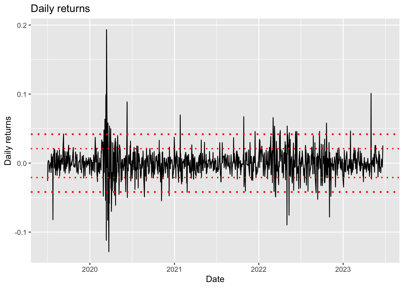
We could plot the returns and the std of returns

library(ggplot2)

ggplot(df |> drop_na(), aes(x = date, y = ret)) + 
  geom_line() + 
  geom_hline(yintercept = stdev, linetype = 'dotted', color = 'red', linewidth= 0.8) + 
  geom_hline(yintercept = -stdev, linetype = 'dotted', color = 'red', linewidth = 0.8) + 
  geom_hline(yintercept = 2*stdev, linetype = 'dotted', color = 'red', linewidth= 1) + 
  geom_hline(yintercept = -2*stdev, linetype = 'dotted', color = 'red', linewidth = 1) + 
  xlab(label = 'Date') + ylab(label = 'Daily returns') + 
  labs(title = 'Daily returns')

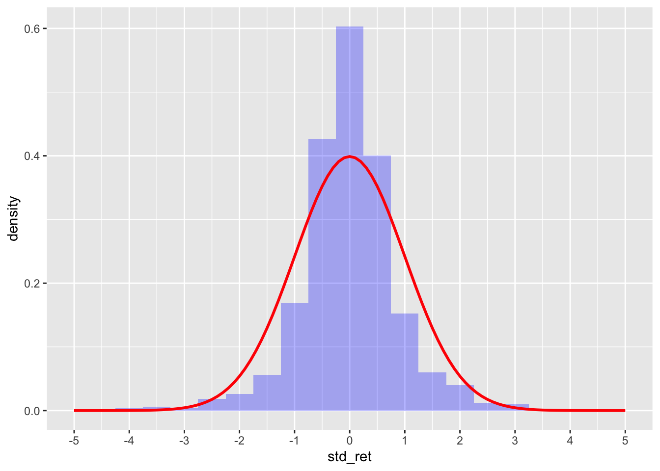
We could standardized the returns (aka ensure they have a mean = 0 and std = 1) and compare it to the standard normal distribution.

df1 <- df |> 
  mutate(std_ret = (ret - r_bar) / stdev) |> 
  drop_na()

ggplot(df1, aes(std_ret)) + 
  geom_histogram(aes(y = ..density..), alpha = 0.3, fill = 'blue', binwidth = 0.5) + 
  stat_function(fun = dnorm, n = 101, args = list(mean = 0, sd = 1), color = 'red', size = 1) +
  scale_y_continuous() + 
  scale_x_continuous(limits = c(-5, 5), n.breaks = 9)

This graph exemplifies what is very common with asset returns: fat tail, and under representation of returns just outside the mean. We discuss this further in our post: The normality of asset returns

The Euler-Maruyana Method to compute the SDE

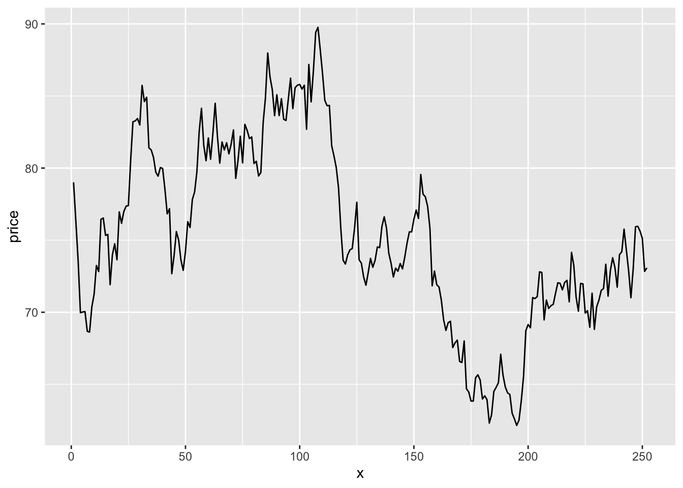
We start with Equation 6 : \(S_{i+1} = S_i \cdot (1 + \mu \delta t + \sigma \phi \sqrt{\delta t})\)

# create one simulation for price 
ndays <- 252 
price <- c()
price[1] <- last(df$adjClose)

phi = rnorm(ndays, mean = 0, sd = 1)

for (i in 2:ndays){ 
  price[i] = price[i-1] * (1 + mu * delta_t + sigma * phi[i] * sqrt(delta_t))
}

yo <- tibble(x = 1:ndays, price = price)
ggplot(yo, aes(x, price)) + 
  geom_line()

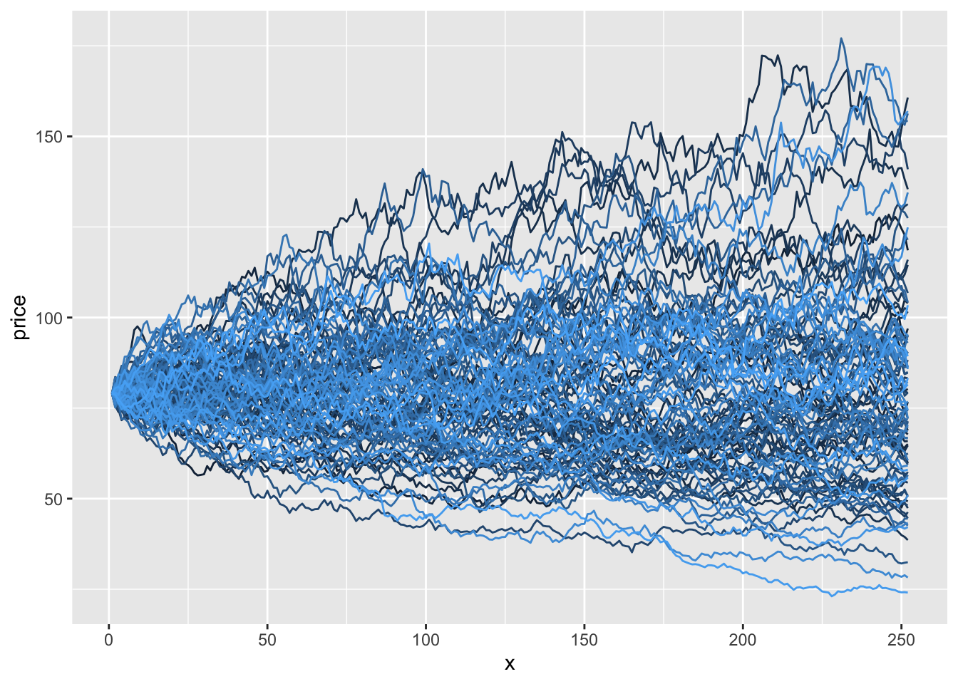
We can now create 100’s such simulations re-using previous code in a function.

create_price_simul <- function(x) {
  price <- c() 
  price[1] <- last(df$adjClose) 
  phi = rnorm(ndays, mean = 0, sd = 1) 
  for (i in 2:ndays){ 
    price[i] = price[i-1] * (1 + mu * delta_t + sigma * phi[i] * sqrt(delta_t)) 
    } 
  yo <- tibble(x = 1:ndays, price = price)
  return(yo)
}

library(purrr)      # map()
library(RColorBrewer)

num_of_simul <- 100
df1 <- tibble(simul_num = 1:num_of_simul) |> 
  mutate(prices = map(simul_num, create_price_simul))

yo <- df1 |> unnest(cols = c(prices))

getPalette = colorRampPalette(brewer.pal(9, "Set1"))
colourCount = num_of_simul
ggplot(yo, aes(x, price, group = simul_num)) + 
  scale_fill_manual(values = colorRampPalette(brewer.pal(9, "Accent"))(colourCount)) +
  geom_line(aes(color = simul_num)) + 
  theme(legend.position = 'none')

Warning in brewer.pal(9, "Accent"): n too large, allowed maximum for palette Accent is 8
Returning the palette you asked for with that many colors