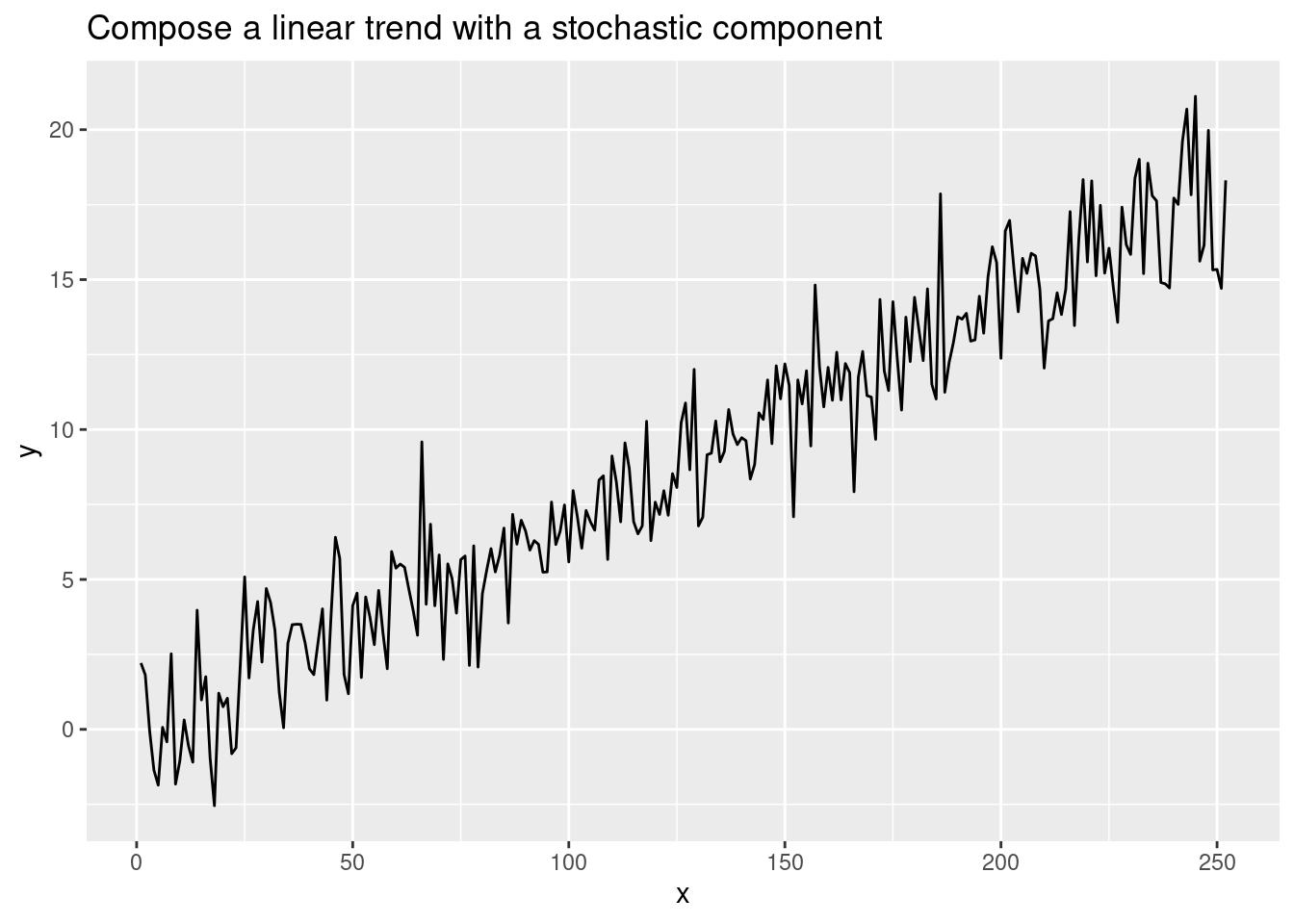
When studying time-series, we usually consider trend and seasonality. With that in mind, we define time-series either in an additive way \[y_t = T_t + S_t + R_t\] or in a multiplicative way \[y_t = T_t \cdot S_t \cdot R_t\]

with

\(y_t\) : the value of the time-serie at time \(t\)
\(T_t\) : the trend component at time \(t\)
\(S_t\) : the seasonal component at time \(t\)
\(R_t\) : the remainder component at time \(t\)

Note

Note that, using log, we can easily transform a multiplicative time-series into an addidiative one.

\[log(y_t) = log(T_t \cdot S_t \cdot R_t) = log(T_t) + log(S_t) + log(R_t)\]

Because decomposition used averages (for seasonal) and noving average (for trend), decomposition is not robust to outlier (aka, it is very sensitive to outlier)

Time-series composition

Perhaps before to decompose time-series, we can try to compose some dummy time-series in both additive or multiplicative ways.

Compose deterministic time-series (with a trend and a stochastic component)

df <- tibble(x = 1:252, phi = rnorm(252, mean = 0, sd = 1.5)) |> 
  mutate(y = 0.07 * x + 0.03 + phi)

ggplot(df, aes(x, y)) + 
  geom_line() + 
  ggtitle(label = 'Compose a linear trend with a stochastic component')

We could also create a seasonal time-series with a stochastic component.

df <- tibble(x = 1:252, phi = rnorm(252, mean = 0, sd = 1.5)) |> 
  mutate(y = 1.7 * sin((2 * pi * x / 50) + 0.3 * pi ) + phi)
         
ggplot(df, aes(x, y)) + 
  geom_line() + 
  ggtitle(label = 'Compose a seasonal trend with a stochastic component')

Decomposing a time-series.

In R using standard library

Let’s go back to the milk example which looks like this.

library(readr)

milk <- read_csv('../../../raw_data/milk.csv')

head(milk)

# A tibble: 6 × 2
  month      milk_prod_per_cow_kg
  <date>                    <dbl>
1 1962-01-01                 265.
2 1962-02-01                 252.
3 1962-03-01                 288 
4 1962-04-01                 295.
5 1962-05-01                 327.
6 1962-06-01                 314.

ggplot(milk, aes(x = month, y = milk_prod_per_cow_kg)) + 
  geom_line()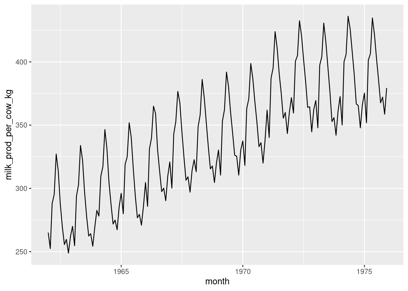

If we transform our tibble into a time-series df, then we can use the decompose() function.

ts_milk <- ts(milk$milk_prod_per_cow_kg, start = c(1962, 1, 1), frequency = 12)
milk_dec <- decompose(ts_milk, type = 'additive', filter = NULL)

plot(milk_dec)

And now, we can use our decomposed time-series to detrend or remove seasonality

milk_adj <- ts_milk - milk_dec$seasonal
plot(milk_adj)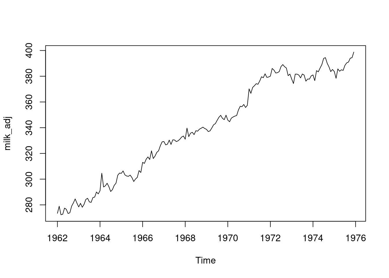

The timtk package can achieve the same output in a more direct way as timetk fit the tidyverse framework.

library(timetk)

milk |> 
  plot_stl_diagnostics(month, milk_prod_per_cow_kg, .frequency = 12)

frequency = 12 observations

trend = 60 observations per 5 years

It should be noted that the timetk package use a Seasonal-Trend-Loess decomposition (STL). If we want to get the values, we use the tk_stl_diagnostics(date, value) function.

(From FPP 3rd ed. )While loess is a method for estimating nonlinear relationships. The STL method was developed by R. B. Cleveland et al. (1990).

STL has several advantages over classical decomposition:

STL will handle any type of seasonality, not only monthly and quarterly data.
The seasonal component is allowed to change over time, and the rate of change can be controlled by the user.
The smoothness of the trend-cycle can also be controlled by the user.
It can be robust to outliers (i.e., the user can specify a robust decomposition), so that occasional unusual observations will not affect the estimates of the trend-cycle and seasonal components. They will, however, affect the remainder component.

head(milk |> tk_stl_diagnostics(month, milk_prod_per_cow_kg))

frequency = 12 observations per 1 year

trend = 60 observations per 5 years

# A tibble: 6 × 6
  month      observed season trend remainder seasadj
  <date>        <dbl>  <dbl> <dbl>     <dbl>   <dbl>
1 1962-01-01     265.  -8.44  272.     1.81     273.
2 1962-02-01     252. -27.2   272.     7.15     280.
3 1962-03-01     288   15.5   273.    -0.726    273.
4 1962-04-01     295.  22.4   274.    -1.18     273.
5 1962-05-01     327.  50.0   275.     2.42     277.
6 1962-06-01     314.  37.3   276.     0.815    276.

Moving averages

There are so many packet in R to calculate moving averages. We’ll keep using the timetk package

yo <- milk |> 
  mutate(ma_3m = slidify_vec(.x = milk_prod_per_cow_kg, .f = mean, .period = 3, .align = 'right'))